Published at February 4, 2026by Benedict Baur

Cluster Analysis in SQL Notebooks and Visualization with Calculation Views

With the SQL Notebook in the Business Application Studio, you can interactively run SQL statements or blocks of SQLScript. This can be used in many ways, for example for data analysis, as an interactive read-me file, or for the setup instructions of an SAP HANA project in CAP. In this blog, I show how to run a cluster analysis in a SQL Notebook. The results are stored in a table and can then be visualized with Calculation Views. Afterwards, I outline the use of HDI containers and the role of SAP HANA's space concept in the context of machine learning.

• SQL Notebook
  • Cluster Analysis in SQLScript
  • Statistical Calculations
  • Aside: AI-supported Interpretation
• Visualization in Calculation Views
• Architectural Considerations - Data Spaces and HDI Containers in SAP HANA
• Summary
• References

First, I would like to motivate the approach:

• SQL Notebook as an extension of the classic SQL console: In the SQL Notebook, the outputs of multiple commands can be saved, whereas in the SQL console you always only see the result of the last execution.
• SQLScript for data analysts: Data analysts like to work with SQLScript (alongside Python). The SQL Notebook allows you to store various analysis scripts in a structured and organized way in a single file in the code repository - without having to create procedures or table functions.
• Interplay with Calc Views: With Calculation Views and the data preview in the Database Explorer (or a BI tool), a wide variety of visualizations of the data analysis result can be created.

SQL Notebook

To use a SQL Notebook, you need an SAP HANA project in the Business Application Studio (or in SAP Build). A SQL Notebook is created as a file with the extension "notebook".

A SQL Notebook consists of several blocks of different types:

• Connection Management: For displaying the available connections and selecting a connection to the HANA database
• Markdown block: Contains text in Markdown. For headings or explanations
• SAP HANA SQL: Contains SQL or SQLScript statements and allows their execution.

First, a block of type Connection Management is created. In this block, the command #List database connections is entered. After execution, the available connections are displayed. To do this, the SQL Notebook reads out the connections assigned to the Cloud Foundry user:

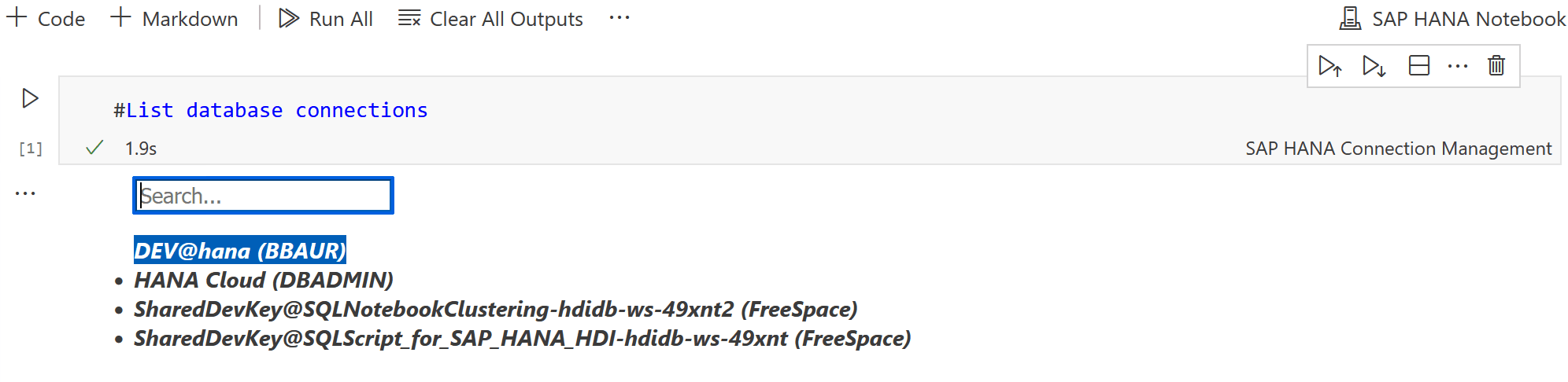
These are the same connections that are assigned to your Cloud Foundry user in the Database Explorer of the HANA Cloud.

In our scenario, you can see:

• two connections to HDI containers (recognizable by SharedDevKey),
• an on-premise connection to HANA Express
• a native connection to the HANA Cloud (with database user DBADMIN without an HDI container). When you select a connection, the connection to the HANA is established.

:nerd_face: Even though the SQL Notebook is a cloud tool, you can connect to an on-premise HANA instance.

To confirm, you can display the current connection to the HANA with the command #Show current database connection:

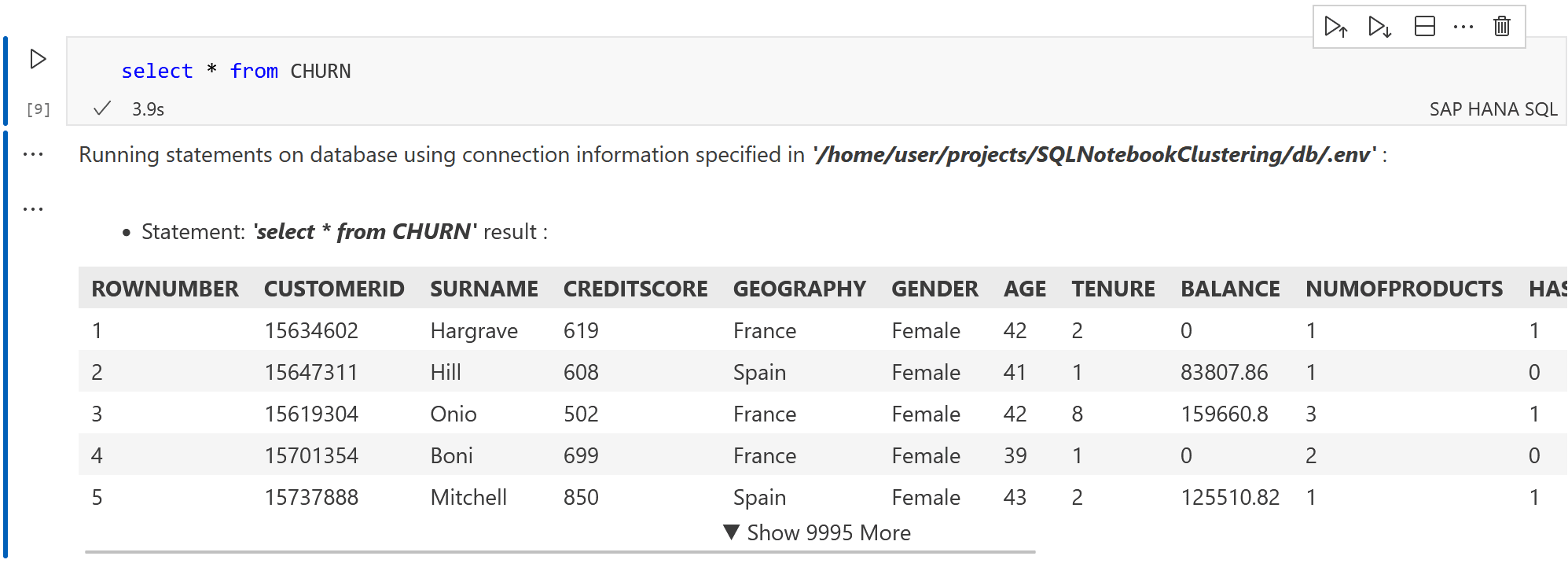
Now you can get started and run your first SQL commands. For the cluster analysis, I use - as in my book - the CHURN dataset (see ¹). It contains 10,000 records of fictitious bank customers. Originally intended for developing a prediction model for churn behavior, I use it here to illustrate a cluster analysis.

Let's start with a simple select statement. To do this, insert a block of type "SAP HANA SQL":

SELECT * FROM CHURN

As a result, you get the table limited to the first rows:

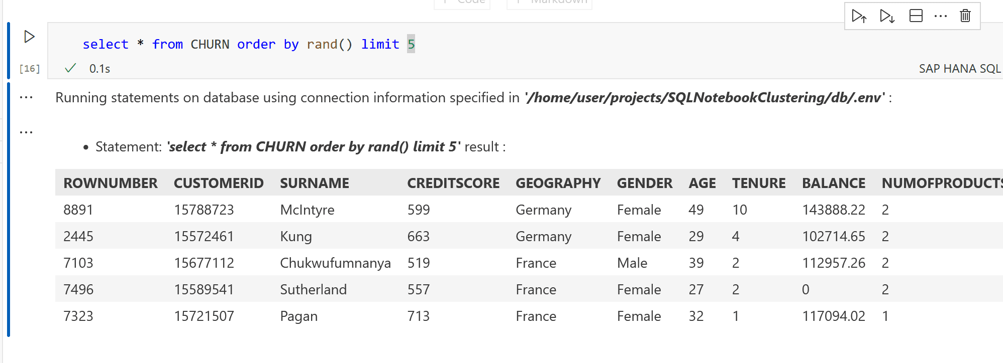
If you want to select a random sample, you can also extend the command:

SELECT * FROM CHURN ORDER BY rand() limit 5

Cluster Analysis in SQLScript

Based on the CHURN table, we now perform the cluster analysis. With a cluster analysis, customers are segmented into groups of similar customers. For the cluster analysis, I use the K-Means algorithm, provided by the PAL procedure _SYS_AFL.PAL_KMEANS. The approach has three parts:

• Building the parameter table for the KMeans procedure
• Calling the procedure
• Storing the cluster assignment in a (container-local) table

This logic must now be encapsulated in an anonymous block. Here I use the source code from my book "Machine Learning mit SAP HANA" (Espresso Tutorial, 2022, ²). For the technical details, I recommend reading my book.

Let's look at the excerpt for building the parameter table:

DO BEGIN
-- Omitted: definition of :lt_parameter 
...

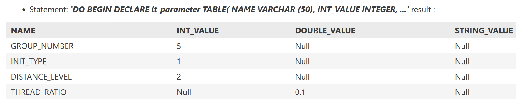
INSERT INTO :lt_parameter VALUES ('GROUP_NUMBER', 5, NULL, NULL);
INSERT INTO :lt_parameter VALUES ('INIT_TYPE', 1, NULL, NULL);
INSERT INTO :lt_parameter VALUES ('DISTANCE_LEVEL',2, NULL, NULL);
INSERT INTO :lt_parameter VALUES ('THREAD_RATIO', NULL, 0.1, NULL);

-- For testing purposes: output
SELECT * FROM :lt_parameter;

END;

Execution yields:

With a SELECT statement, we select the relevant columns that should be chosen as input features for the clustering. Different selections of features lead to different cluster results. At the same time, we extend the anonymous block with the call of the cluster procedure:

lt_churn = SELECT CUSTOMERID,
				  GEOGRAPHY,
				  AGE,
				  TENURE,
				  BALANCE,
				  NUMOFPRODUCTS,
				  ESTIMATEDSALARY
				  FROM CHURN WHERE BALANCE > 0;


CALL _SYS_AFL.PAL_KMEANS(:lt_churn, 
                          :lt_parameter, 
                          lt_result, 
                          lt_centers, 
                          lt_model, 
                          lt_statistics, 
                          lt_placeholder);

The cluster assignment is output in lt_result, the cluster centers in lt_centers. By appending a select command in the anonymous block, the cluster assignment is output after execution:

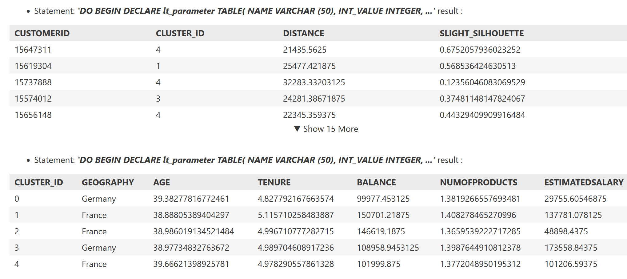
To use the cluster assignment for further analyses, we store it after execution in the (container-local) table CLUSTER_RESULT.

:💡 : Difference between Python and SQL Notebook

Unlike in a Jupyter Notebook for Python, no local variables are defined in a SQL Notebook. The blocks form independent units that only share the common database connection. An exchange of information between the blocks is therefore only possible via session variables or temporary tables. In the example shown here, I use a persistent table CLUSTER_RESULT that I defined in a HANA project as an hdbtable file. This is then deployed as a container-local table.

Statistical Calculations

To analyze the distribution of the numerical attributes by cluster more precisely, you can calculate means and percentiles. The percentiles can be computed in SQLScript as a window expression with the window aggregation function percentile. The following code block first selects the result of the cluster analysis with RUN_ID = 1 and then performs the percentile calculation:

DO BEGIN 

lt_customer_cluster = SELECT c.customerid, 
                             r.cluster_id, 
                             c.age, 
                             c.balance FROM CHURN as c JOIN cluster_result as r on c.CUSTOMERID = r.CUSTOMERID
                             where r.RUN_ID = 1;

lt_percentile = SELECT customerid, cluster_id, age, balance,
    PERCENTILE_CONT(0.25) WITHIN GROUP (ORDER BY age) OVER (PARTITION BY cluster_id) AS age_p25,
    PERCENTILE_CONT(0.50) WITHIN GROUP (ORDER BY age) OVER (PARTITION BY cluster_id) AS age_p50, 
    PERCENTILE_CONT(0.75) WITHIN GROUP (ORDER BY age) OVER (PARTITION BY cluster_id) AS age_p75, 
    PERCENTILE_CONT(0.25) WITHIN GROUP (ORDER BY balance) OVER (PARTITION BY cluster_id) AS balance_p25,
    PERCENTILE_CONT(0.50) WITHIN GROUP (ORDER BY balance) OVER (PARTITION BY cluster_id) AS balance_p50,
    PERCENTILE_CONT(0.75) WITHIN GROUP (ORDER BY balance) OVER (PARTITION BY cluster_id) AS balance_p75 from :lt_customer_cluster;
     

SELECT cluster_id, max(age_p25) as age_p25, 
                   max(age_p50) as age_p50,
                   max(age_p75) as age_p75, 
                   avg(age) as mean_age,
                   max(balance_p25) as balance_p25, 
                   max(balance_p50) as balance_p50, 
                   max(balance_p75) as balance_p75,
                   avg(balance) as mean_balance
                   FROM :lt_percentile group by cluster_id order by cluster_id;


END;

Result:

💡 The Percentile Cont function is a so-called window aggregate function: Within the defined partition (here the clusters), an aggregation is calculated and the aggregated value is written to each row of the partition. However, the percentile functions are not available in an ordinary aggregation with a Group By statement.

• The result can be interpreted as follows: The age distribution does not differ between the clusters (the middle 50% lie in the range 32 - 45).
• The distribution for balance (account balance) differs between the clusters:
  • Clusters 0 and 4 contain the customers with lower account balances.
  • Clusters 1 and 2 contain customers with higher account balances.

Other segmentations of the customers can be obtained by reducing the input data to certain features or by using a normalization of the features. In the SQL Notebook (see the GitHub project: ³ ), another cluster configuration is listed in which segmentation is done only by age and credit score, and in addition the input variables are normalized beforehand.

Aside: AI-supported Interpretation

While writing this blog, I - more for fun - copied the cluster-aggregated output of the previous section into Microsoft Copilot as a prompt. This is what came out:

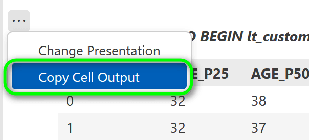
🤓 You can copy the tabular output of the statistical metrics as a JSON array using the "Copy Cell Output" function. You can enter this string 1:1 into Microsoft Copilot. Microsoft Copilot then independently performs an interpretation of the cluster results (based on the summarized statistical metrics) and even allows visualization of the clusters.

Processing by Copilot/ChatGPT:

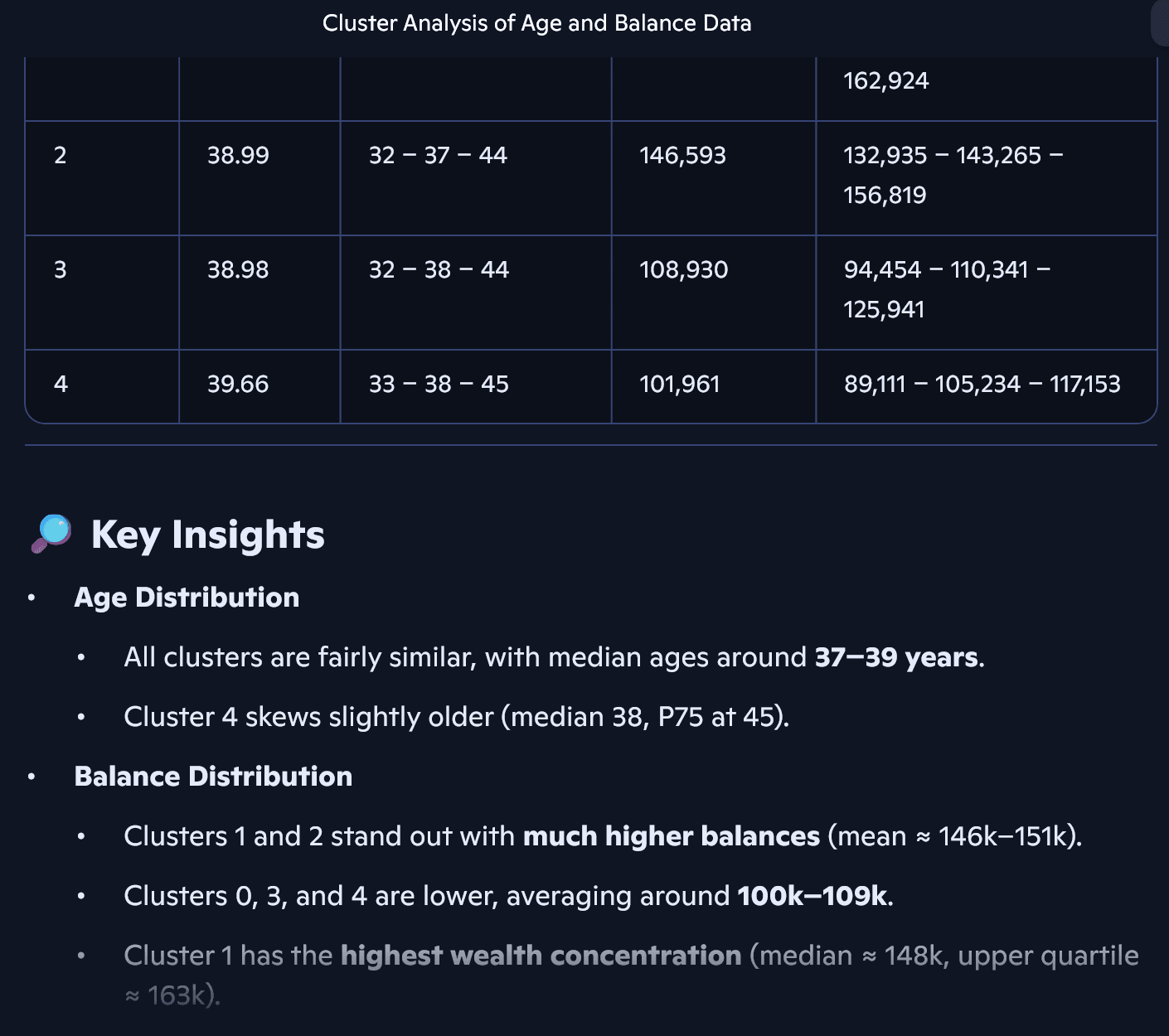
The key point: The statistical calculations already take place in SAP HANA (by executing the SQL statement above) - lightning fast thanks to in-memory. Copilot here only has to process the calculated statistical metrics, which corresponds to a highly aggregated and consequently very small dataset. In particular, no individual customer records have to be delivered from the SAP system to Copilot.

Visualization in Calculation Views

Now that we have run the cluster analysis via SQLScript, it can be further examined and visualized using Calculation Views.

In my last blog⁴, I already showed some visualizations:

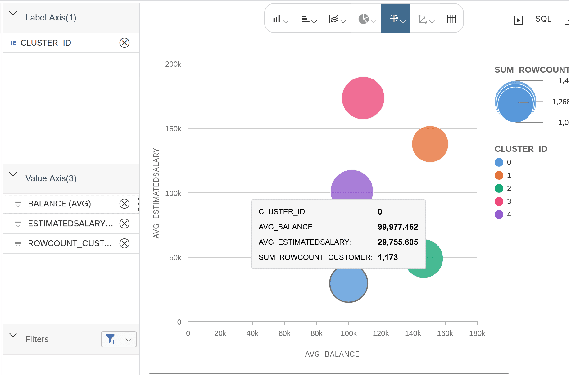
• Bubble chart for the cluster centers
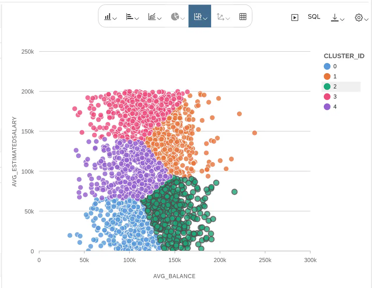
• Scatter plot with a random sample per cluster

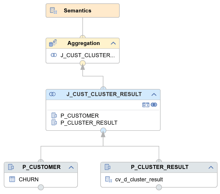
The basic modeling consists of linking the source table CHURN (with the customer data) to the result table for the cluster assignments CLUSTER_RESULT via a JOIN.

The following figure shows the basic form of the Calculation View:

Visualization of the cluster centers as a bubble chart:

Scatter plot with a random sample per cluster:

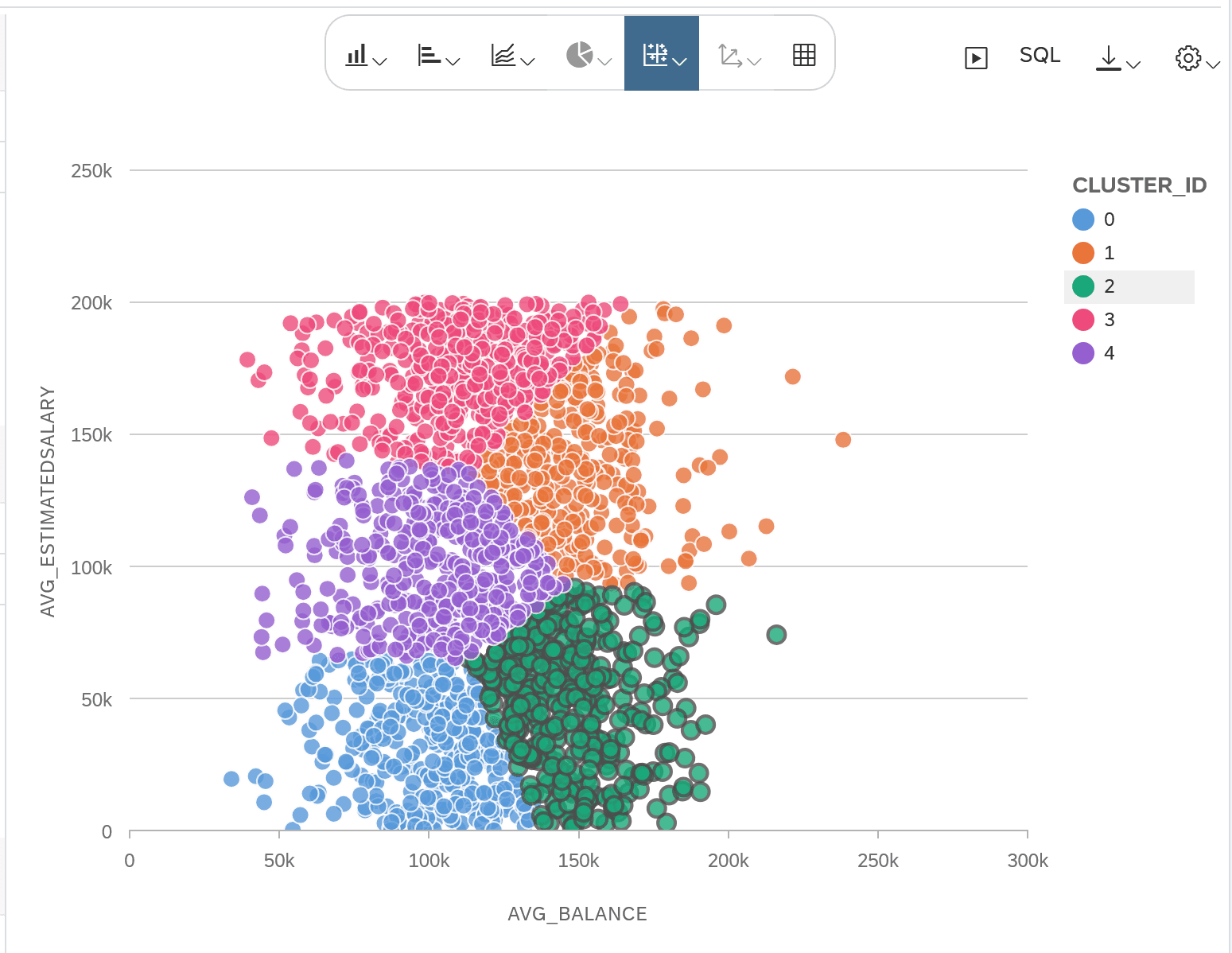
How to model the random sample using the Window Function node type, I described in my last blog⁴.

I would now like to introduce another helpful technique for the analysis, so-called binning: The age column (AGE) can be discretized using the window function NTILE, i.e. a categorical column can be created that assigns each record to an interval based on age, or each customer to an age group. This can be used to analyze the distribution of customers in the individual clusters by age group.

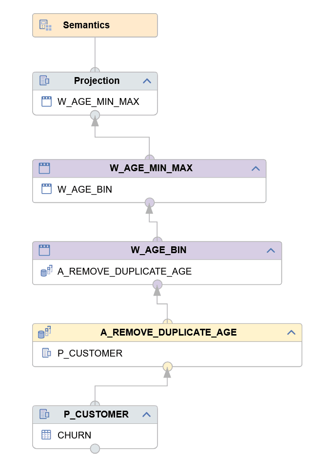
To create the discrete column AGE_BIN, I create the dimension view CV_D_AGE_BINNING, which has the following structure:

{height = 500px}

The individual nodes have the following function:

• Aggregation node A_REMOVE_DUPLICATE_AGE: By aggregating on the AGE column (as an aggregation characteristic), the distinct values of the AGE column are selected. In SQL, this corresponds to SELECT DISTINCT.
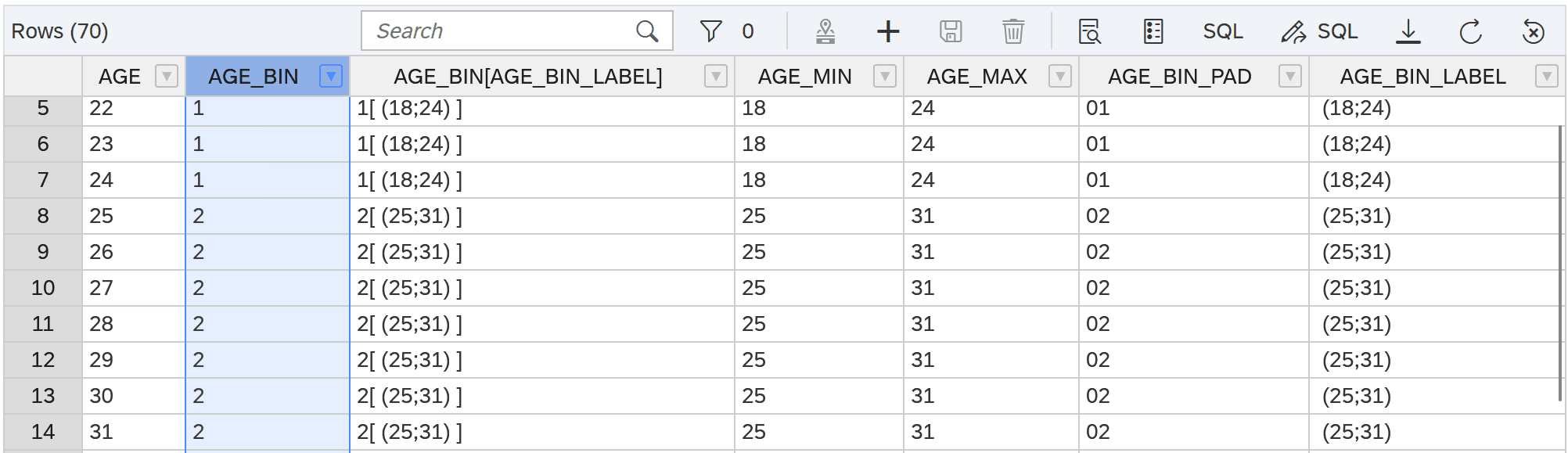
• Window Function node W_AGE_BIN: Uses the function N_TILE to divide the value range of AGE into intervals. Each value for AGE is assigned to a group. This assignment forms the new column AGE_BIN.
• Window Function node W_AGE_MIN_MAX: Calculates the minimum and maximum age per group (AGE_BIN).
• Projection: Output of the columns and additional calculation of the interval label AGE_LABEL.

The modeling of the window function in the node W_AGE_BIN looks like this:

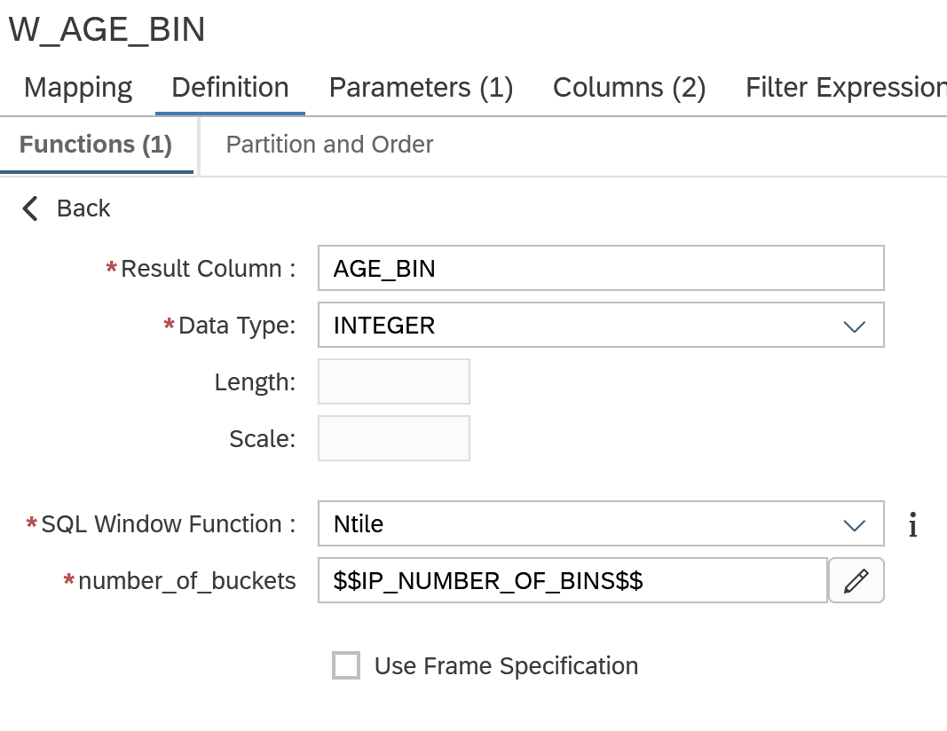
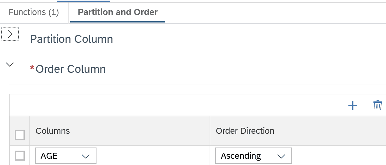
• The records are sorted by AGE (set in the Partition and Order tab).
• The window function Ntile then forms groups of records according to the sorting.
• The number of groups to be formed is defined via the number_of_buckets setting. We supply this via the input parameter IP_NUMBER_OF_BINS.

A sample output for IP_NUMBER_OF_BINS = 10 looks like this:

Now the previously modeled cube view (linking customer attributes and cluster assignment) can be extended with a join to the dimension view CV_D_AGE_BINNING. The number of customers can now be counted per cluster and age group. We consider the visualization for IP_NUMBER_OF_BINS = 5.

For example, the following bar chart compares the age distribution in clusters 0, 1 and 3:

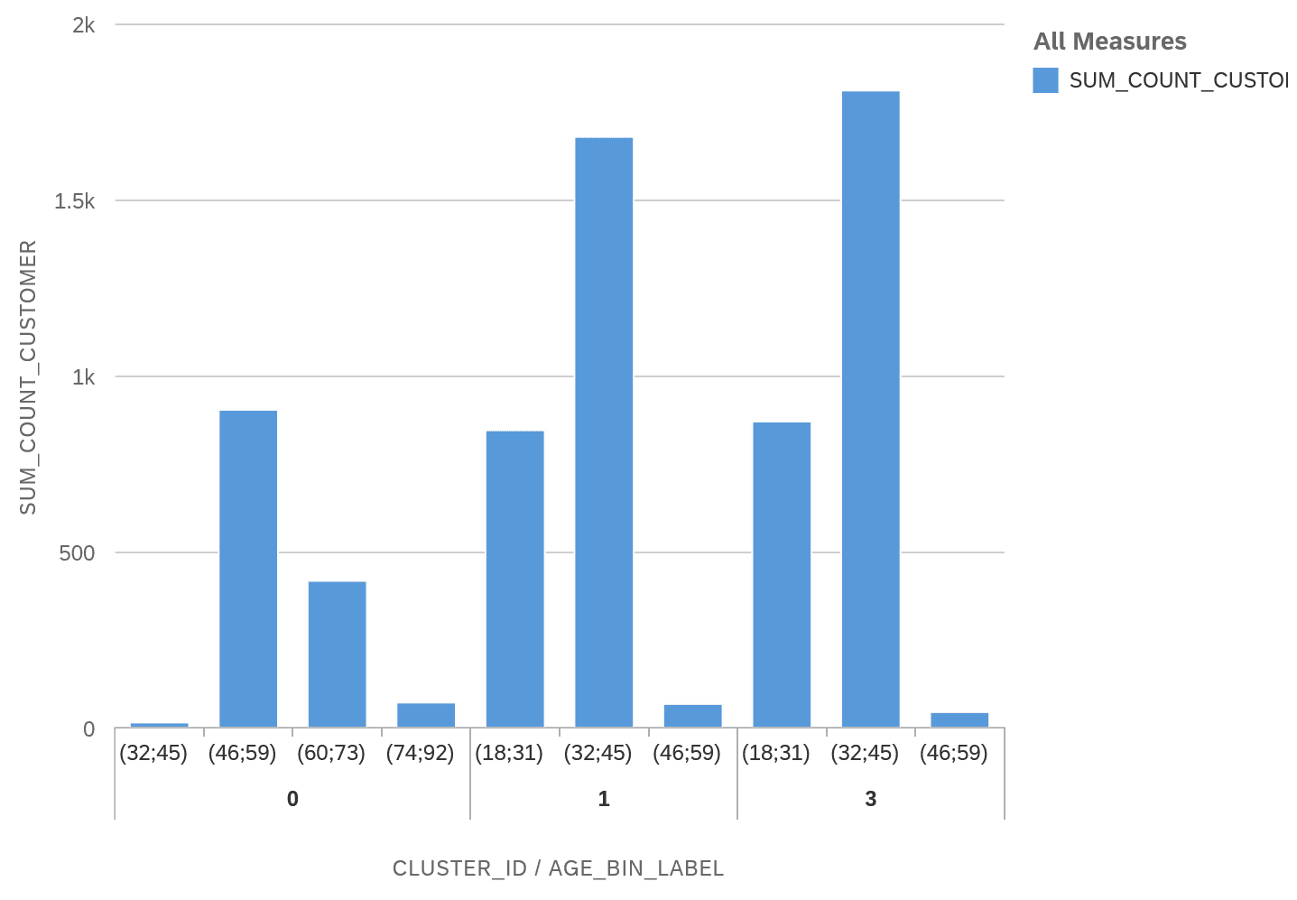
It can be seen that in cluster 0 the age groups 46-59, 60-73 and 74-92 are represented, whereas in clusters 1 and 3 the age groups 18-31 and 32-45 dominate.

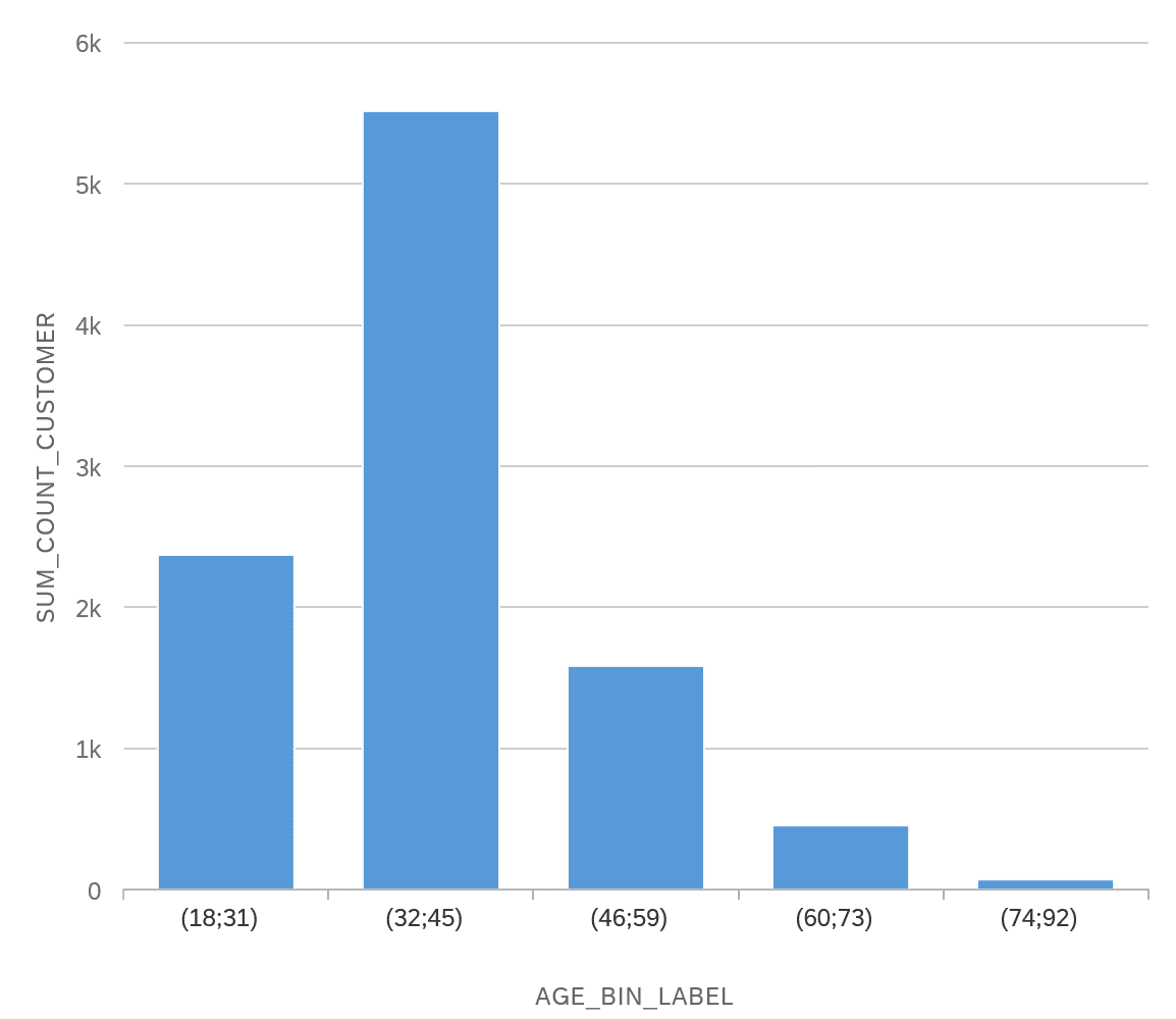
For comparison, you can also look at the age distribution across the entirety of the customers:

Architectural Considerations - Data Spaces and HDI Containers in SAP HANA

In this chapter, I would like to address why the use of data spaces and HDI containers in SAP HANA is helpful for the successful use of machine learning.

The process of developing machine learning models or ML-supported data analyses requires, among other things, two conditions:

• Access to productive real data - possibly anonymized and historized.
• The possibility to create HANA artifacts (Calculation Views, stored procedures, etc.) and to store intermediate results.

The classic three-system environment of an SAP landscape consisting of development system, test system and production is therefore only suitable for machine learning with limitations. This is where the use of spaces comes into play, which can be created either natively in SAP HANA or in Datasphere. A space is an isolated environment in HANA with its own authorization management and control of resource usage. When deploying an HDI container, you select which space the container should be deployed to.

The following figure shows the use of spaces in the context of machine learning:

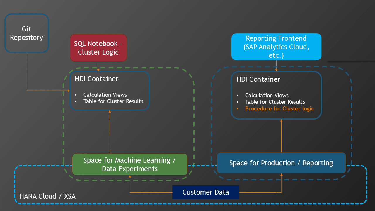
On a production system, a dedicated "Green space" for machine learning can be set up. The data scientist or machine learning developer is assigned appropriate authorizations in this Green Space. The blue box "Customer Data" here symbolizes the customer data that is used as input data for the cluster analysis. Access to already existing data is provided by appropriate External Services. In principle, this corresponds to a technical database user. By limiting the CPU and memory usage of the Green space, the production system is prevented from being overly burdened by the execution of the machine learning algorithms.

For developing database artifacts, the HDI containers (in XSA or HANA Cloud) are ideal:

• Each ML developer can first deploy their development in their own container.
• Intermediate results are stored in container-local tables.

Merging developments can then take place centrally via a Git repository.

As soon as a suitable analysis approach - consisting of data preparation, selection of the relevant features and a suitable cluster algorithm - has been found, the machine learning logic can be consolidated in a database procedure. The procedure and Calculation Views for evaluation can then be deployed to the central production space. There, the cluster procedure can then be run regularly. The cluster results are then directly available for consumption in reporting via the Calculation Views.

Thanks to XSA, this scenario can also be realized in an on-premise environment without Data Sphere.

Summary

I leave the summary of this article to ChatGPT (Smart GPT-5) - with minor corrections:

• The SQL Notebook in SAP Business Application Studio enables interactive data analyses with SQLScript and offers, compared to the classic SQL console, the advantage of storing the results of multiple commands in a structured way.
• Using a dataset of fictitious customers, it was shown how a cluster analysis is performed with the K-Means algorithm and how the results can be persisted in a table.
• In addition, statistical calculations such as percentiles and means can be executed directly in SQLScript to characterize the clusters in more detail.
• With Calculation Views, the results can then be visually prepared, for example through bubble or scatter charts as well as through techniques such as binning to analyze age groups.
• Architecturally, HDI containers and spaces in SAP HANA play a central role, as they create isolated environments for machine learning developments and ensure access to productive data as well as resource control.

References

Footnotes

1. Churn modeling from Kaggle: https://www.kaggle.com/datasets/shivan118/churn-modeling-dataset ↩

2. My book: https://es-tu.de/e9ZD2 ↩

3. GitHub repository: https://github.com/drabap/SQLNotebookClustering ↩

4. https://www.brandeis.de/blog/2025-cluster-analysen-calculation-views/ ↩ ↩²