Published at February 12, 2025by Benedict Baur

Machine learning logic implemented in SQLScript can be integrated into calculation views by using table functions. With the new snapshot function for calculation views in the Business Application Studio, the results of the machine learning execution can be stored and used for advanced analyses in calculation views. I demonstrate the approach using a segmentation of customer data with the PAL procedure for the K-Means cluster algorithm.

Note: I presented the approach shown here in a live demo at the HANA Tech Night in June 2024, see: https://www.brandeis.de/blog/events/htn-10-recap.

• New functions in calculation views and architecture sketch
• Implementing the table function with the cluster logic
• Integrating the table function in the calculation view
• Using the snapshot function
  • Activating the snapshot function
  • Structure of the interface view and parameter passing
  • Objects created in the database
• Integration into a cube calculation view for further analysis
  • Scatter chart and window functions
• Conclusion and outlook

Note: My GitHub repository https://github.com/drabap/CalcViewClustering contains the table function for the cluster logic and a simple calculation view. With it you can reproduce the examples in this blog.

New functions in calculation views and architecture sketch

Motivation: A cluster analysis allows you to identify structures and relationships in data. In the example considered here, a set of customer data is segmented. This makes it possible, for instance, to identify interesting customer groups.

The following functions, which are available when modeling calculation views in the Business Application Studio, prove useful in this context and are used or shown in this blog:

• Table functions with a table input parameter (already available in the Web IDE, but not in Eclipse)
• Snapshot creation
• Window functions

The architecture looks like this:

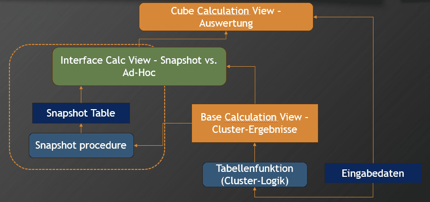
The architecture sketch shows the following components:

• Input data: The data to be used as input for the cluster analysis. In our case, the customer data.
• Table function: This function implements the cluster logic and returns the cluster assignments in a table.
• Base Calculation View - Cluster results: This calculation view calls the table function and thereby triggers the execution of the cluster procedure.
• Snapshot Table: Generated table for storing a snapshot of the base calculation view. This is where the results of the cluster assignment are stored.
• Snapshot Procedure: Generated procedure for executing the base calculation view and storing the results.
• Interface Calc View: Generated view that provides both access to the base view (for an ad-hoc execution of the cluster analysis) and to the snapshot.
• Cube Calculation View - Evaluation: In this calculation view, the cluster assignments (from the snapshot or the base view) are enriched with the customer attributes. This view thus enables further analysis of the cluster results in the context of the customer attributes.

Implementing the table function with the cluster logic

First, I implement the table function for executing the cluster logic. Hyperparameters of the cluster algorithm can be provided as input parameters. For the sake of simplicity, I only consider the two hyperparameters:

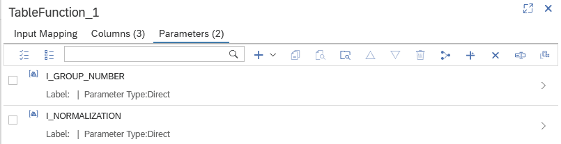
• I_GROUP_NUMBER: Number of clusters/groups to be formed
• I_NORMALIZATION: Rescaling of the input data.

Using the input parameters, a parameter table (lt_parameter) is first built, containing the parameter values. This is passed, together with the input data (lt_customer - the customer data for the segmentation), to the PAL procedure of the cluster algorithm:

CALL _SYS_AFL.PAL_KMEANS(:lt_customer, 
                         :lt_parameter, 
                         lt_result, 
                         lt_centers, 
                         lt_model, lt_statistics, lt_placeholder);

The return table of the table function should contain the following columns:

• CUSTOMERID: Customer number for the unique identification of the source record.
• DISTANCE: Distance of the record from the assigned cluster center.
• CLUSTER_ID: Number of the assigned cluster.

The return is built from the table variable lt_result:

return select customerid,
              distance, 
              cluster_id
        from :lt_result;

You can find the complete source code of the table function in the GitHub repository already mentioned: https://github.com/drabap/CalcViewClustering/blob/main/db/src/tbl_fun_cluster_tab_input_inp_par.hdbfunction.

For an overview of the possible hyperparameters and the details of the implementation in SQLScript, I refer to my book "Machine Learning mit SAP HANA" (https://es-tu.de/e9ZD2)

Integrating the table function in the calculation view

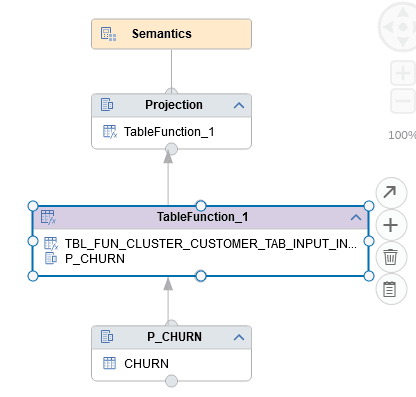
A table function can be used directly as a data source in a calculation view. In the web-based modeling there is a dedicated node type "Table Function", which even supports table functions with a table input parameter. In our example, the table function TBL_FUN_CLUSTER is added to the node TableFunction_1.

The input data for the clustering is supplied via a projection node. This node selects from the table CHURN (which contains the customer data):

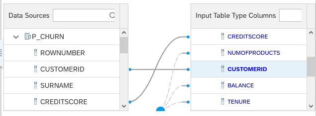
On the "Input Mapping" tab, the columns of the projection node (table CHURN) are mapped to the columns of the input parameter IT_INPUT of the table function:

On the Parameters tab of the node TableFunction_1, input parameters for the calculation view can be created directly from the scalar input parameters of the table function:

After the usual modeling steps (adding fields to the output, etc.), the calculation view can be executed in the Data Preview:

After entering the parameters ...

... the cluster logic is executed:

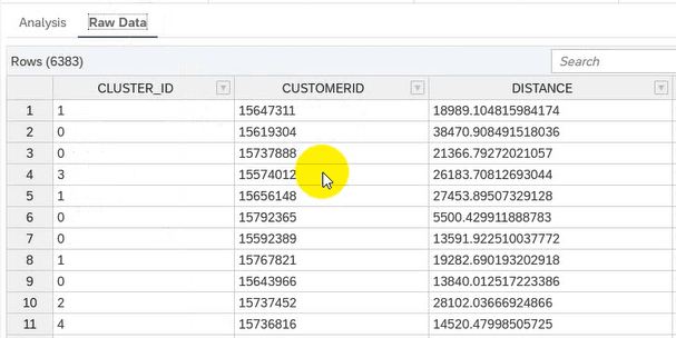
While direct execution is helpful when experimenting, it has the disadvantage that the entire cluster logic is run through again with every navigation step in the data preview. This has a negative impact on runtime and resource consumption. In addition, the cluster algorithm contains random elements, e.g. the initialization of the cluster centers. This can lead to a different result with every execution.

This is where the new snapshot function comes into play, which I will now examine.

Using the snapshot function

The snapshot function was introduced a few releases ago in the modeling with Business Application Studio (BAS). The basic idea is to store the result set of queries defined on the calculation view in a table and to make these results available for later use.

Activating the snapshot function

The snapshot function is activated in the semantics node. You can define one or more queries. Since the calculation view here is a simple dimension view without aggregation, we make a simple SELECT statement with a complete projection clause. The queries are defined on the Snapshots tab in the semantics node:

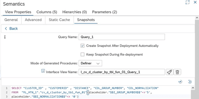
The following important points can be seen here:

• The snapshot is defined via an SQL query. When using input parameters, it is important to specify them explicitly in the SQL query. This way the input parameters are also exposed by the generated procedures for managing the snapshot.
• An interface view is generated (field Interface View Name). This allows both access to the data stored in the snapshot and to the underlying base view.
• With the option "Create Snapshot After Deployment Automatically", you can trigger the snapshot creation when the view is deployed. This is particularly helpful in iterative development.

In the backend, a table is created to store the snapshot. I will show how to read it using the interface view in the next section.

Structure of the interface view and parameter passing

The automatically generated interface view is created by the BAS as a design-time object and can thus be integrated into further calculation views of your own.

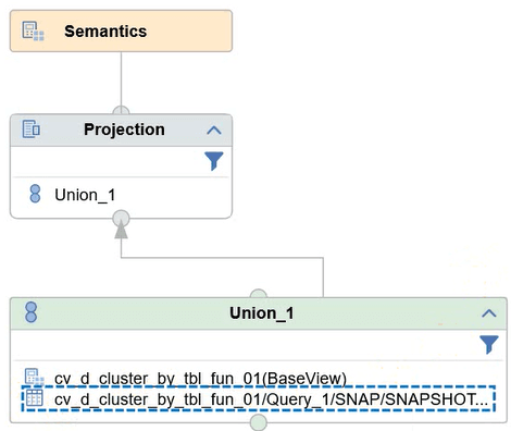
The interface view consists of a union of the snapshot table and the original calculation view. The interface view has the input parameter I_SOURCE. This allows you to determine the data source at runtime:

• BASE: Selection from the base view.
• SNAPSHOT: Reading the snapshot.

In our scenario, BASE thus corresponds to the ad-hoc execution of the cluster logic, while SNAPSHOT corresponds to reading the cluster assignment from a previous run.

With this input parameter, a filtering takes place on the input nodes of the union node. Thanks to UNION pruning, it is guaranteed that only one of the two input nodes is ever executed.

So that the input parameters of the table function can also be supplied by the interface view, they must be mapped manually in the interface view. Note here that an adjustment of a generated object takes place. If the snapshot query is changed and the interface view is regenerated, these adjustments must therefore be repeated:

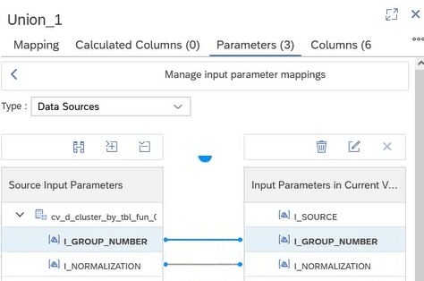
To also take the input parameters into account when reading the snapshot, I applied the following trick:

• The return of the base view (call of the table function) contains the input parameters as a constant column.
• In the projection node of the interface view, I defined a filter expression for these columns with the current values of the input parameters:

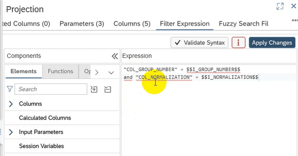
Here is the filter expression as a code snippet:

"COL_GROUP_NUMBER" = $$I_GROUP_NUMBER$$
and "COL_NORMALIZATION" = $$I_NORMALIZATION$$

The filter expression ensures that only the snapshot matching the input parameters is read. When calling the base view, the filter has no effect, since the base view returns the values of the input parameters in the two columns.

Let us look at the interface view in the data preview. We call the interface view with the parameter selection I_SOURCE = SNAPSHOT and the default values I_GROUP_NUMBER = 5 and I_NORMALIZATION = 0, which were specified in the defining query:

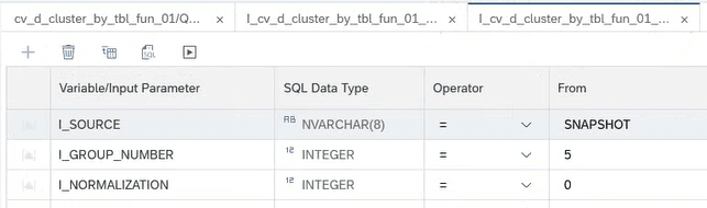
With this selection, we get the rows from the snapshot that was automatically created during deployment:

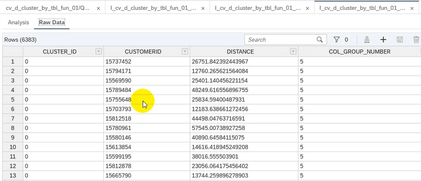
How you can store snapshots of further executions in the table after deployment I will show in the next section.

Objects created in the database

The snapshot function creates the following objects (in addition to the column views of the calculation views):

• Snapshot table for storing the snapshot
• Procedures for managing the snapshot.

The snapshot table has as its structure the field list of the defining query:

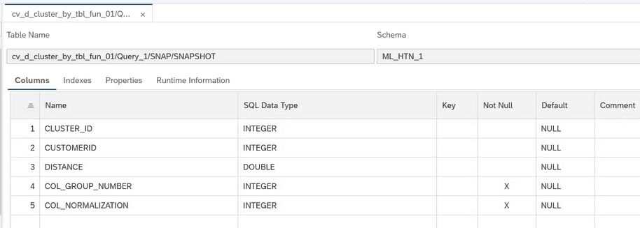
In addition to the columns of the return of the table function, the two constant columns for the input parameters can be seen (COL_GROUP_NUMBER and COL_NORMALIZATION). As mentioned above, I manually inserted a filter expression for these columns in the interface view.

The following procedures are created:

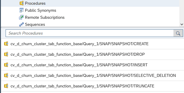
• CREATE: Create and populate the snapshot table (after deletion)
• INSERT: Insert a new snapshot into the table
• DROP: Delete the snapshot table
• SELECTIVE_DELETION: Selective deletion of snapshot entries using a dynamic filter (new in the September 2024 release)
• TRUNCATE: Truncate the snapshot table (delete + commit)

An example flow could look like this:

• With the INSERT procedure, further runs of the cluster algorithm are executed with different input parameters.
• With the DROP procedure, the snapshot table is completely deleted if needed and can be rebuilt with the CREATE procedure.

It would also be conceivable to run the INSERT procedure regularly, for example via scheduling in SAP HANA. Old snapshots can then be specifically removed via the SELECT_DELETION procedure.

This screenshot shows the signature of the INSERT procedure:

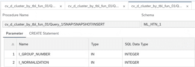
As you can see, the two input parameters of the table function and of the calculation view are offered. Thus, several cluster runs can be executed with different parameter values and stored in the snapshot.

If we now run the INSERT procedure for the new parameter combination GROUP_NUMBER = 5 and NORMALIZATION = 2, we now also see records for the new parameter combination in the snapshot table:

CALL "HANA_CLUSTER_TABLE_FUNCTION_CALC_VIEW_HDI_DB_1".  
"cv_d_churn_cluster_tab_function_base/Query_1/SNAP/SNAPSHOT/INSERT"(I_GROUP_NUMBER => 5 ,
I_NORMALIZATION => 2)

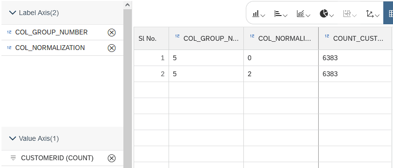
The number of records of 6383 per combination corresponds exactly to the number of selected customers for the cluster execution (customers with BALANCE = 0 were excluded).

Integration into a cube calculation view for further analysis

In order to be able to interpret the results of the cluster algorithm, the cluster assignments of the individual customers must be related to the input data, the attributes of the customers. To do this, I integrate the interface view into a calculation view of type Cube. Using the interface view makes it possible to perform the further analyses both with data from the snapshot and with an ad-hoc execution of the cluster logic, while using the same calculation view.

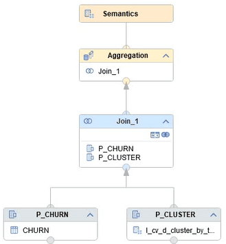
The calculation view for the analysis is structured as follows:

• Via projection nodes, the customer data (CHURN) and the interface view are integrated respectively.
• The two data sources are linked via a JOIN along the customer number (column CUSTOMERID).
• In the top aggregation node, a counter for the customers is defined.

This is what the structure of the calculation view looks like:

In the semantics node, the following settings are made:

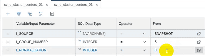
• The input parameters of the interface view are made available as input parameters in the calculation view via "Parameter Mapping".
• The numeric attributes of the customers are defined as key figures; the text-type attributes, or numeric attributes that are to be regarded as a categorical characteristic, are defined as characteristics.

In the data preview, you now have the choice between the snapshot and the base view:

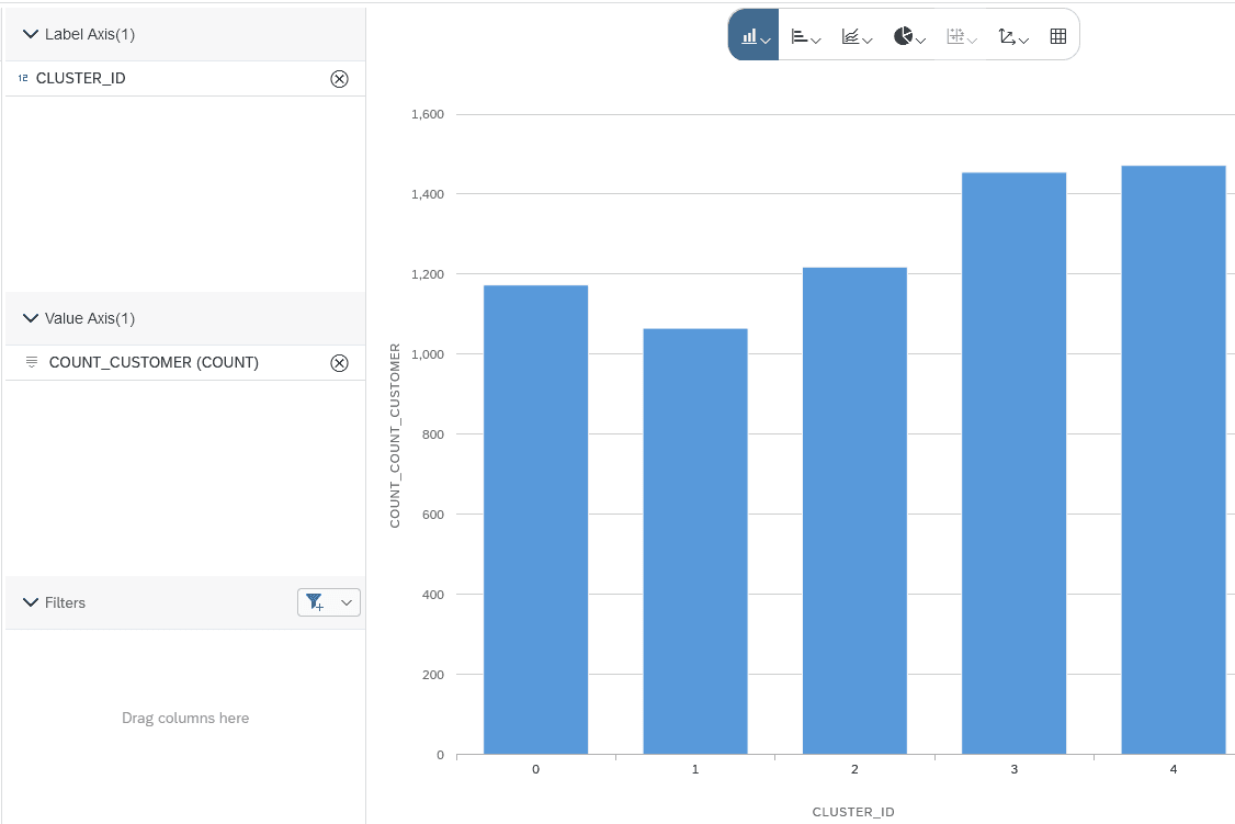
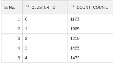
If you aggregate the key figure COUNT_CUSTOMER by the clusters, you can count the number of customers per cluster:

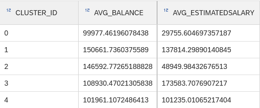
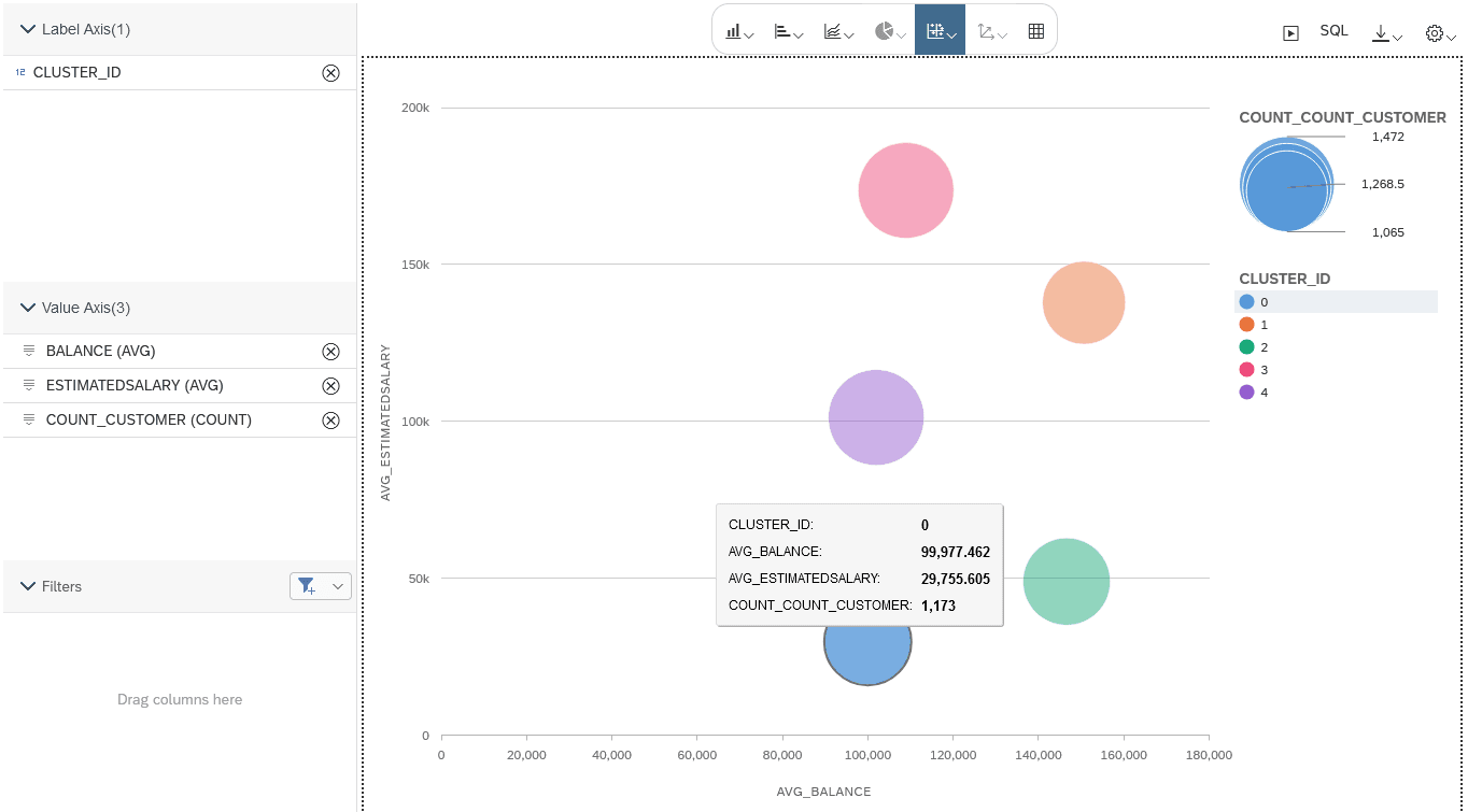
With the numeric attributes of the customers, you can now draw a bubble chart to estimate the position of the cluster centers. As the aggregation function we choose AVG (average):

The size of the bubbles is determined by the number of customers per cluster:

Scatter chart and window functions

The cube calculation view can now be extended as desired to perform more complex analyses of the customer structure by clusters. The new node type Window Function in the BAS also proves helpful here.

The node type Window Function can be used, for example, for the following scenario:

Scatter chart by customer with random sampling:

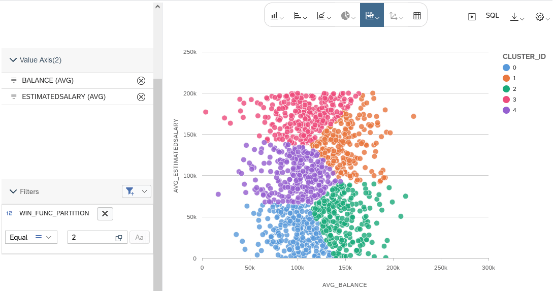
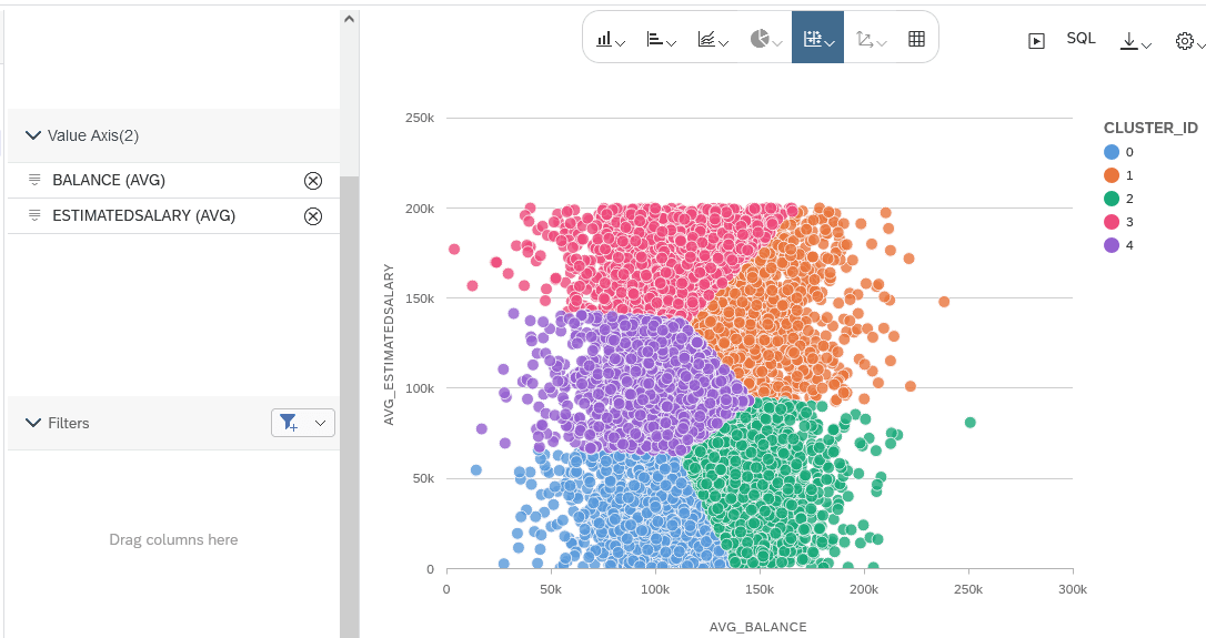
• If, in the example above, you add the customer number (CUSTOMER_ID) to the layout in addition to the CLUSTER_ID, you get a scatter chart with all customers, colored by the cluster assignment.
• However, this means the result set contains a very large number of records - each point in the scatter chart corresponds to one customer.
• With the window function Random partition, a random sample can now be drawn per cluster. This reduces the number of records in the result again and still makes it possible to estimate the shape of the clusters.

For this, the calculation view is extended as follows: A "Window Function" node is inserted above the JOIN node:

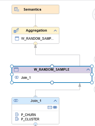
In the node, the window function "Random Partition" is selected.

This window function is used to divide a data set into two or three random subsets. This function is actually used in supervised learning (e.g. for classification problems). We use it here to obtain a subset of the result set:

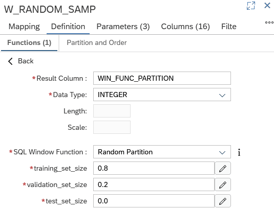
It works as follows: A column WIN_FUNC_PARTITION is created. Each record is randomly assigned to the subset "Training Set" (80%) or the subset "Validation Set" (20%). The assignment can be recognized by the value of the column WIN_FUNC_PARTITION. To perform the random sampling per cluster, the column CLUSTER_ID must be assigned to the partition:

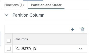
This approach is also called stratified sampling.

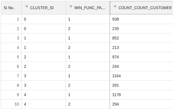
Aggregation by CLUSTER_ID shows that per cluster approx. 80% of the records are assigned to set 1 (Training) and 20% of the records to set 2 (Validation):

In the scatter chart, you can now lay out by customer and additionally filter by the subset, e.g. the 20% subset:

For comparison, the scatter chart without filtering:

Conclusion and outlook

In this blog, I showed how, using SQLScript with table functions, machine learning logic can be integrated into calculation views. Using the new snapshot function makes it possible to store the result of the cluster execution for later analyses. This allows the two scenarios of ad-hoc execution and batch execution of the machine learning logic to be combined with one modeling tool. New modeling functions of calculation views in the Business Application Studio, such as window functions, enable further analyses.

If you integrate the calculation view into the SAP Analytics Cloud, the cluster results can be used by reporting users. The procedures for snapshot management can be executed manually or scheduled via scheduling services in SAP HANA.